Cococubed.com Slow Neutron Captures
Home Astronomy Research    2024 Radiative Opacity    2024 Neutrino Emission from Stars    2023 White Dwarfs & 12C(α,γ)16O    2023 MESA VI    2022 Earendel, A Highly Magnified Star    2022 Black Hole Mass Spectrum    2021 Skye Equation of State    2021 White Dwarf Pulsations & 22Ne    Software Instruments      Stellar equation of states      EOS with ionization      EOS for supernovae      Chemical potentials      Stellar atmospheres      Voigt Function      Jeans escape      Polytropic stars      Cold white dwarfs      Adiabatic white dwarfs      Cold neutron stars      Stellar opacities      Neutrino energy loss rates      Ephemeris routines      Fermi-Dirac functions      Polyhedra volume      Plane - cube intersection      Coating an ellipsoid      Nuclear reaction networks      Nuclear statistical equilibrium      Laminar deflagrations      CJ detonations      ZND detonations      Fitting to conic sections      Unusual linear algebra      Derivatives on uneven grids      Pentadiagonal solver      Quadratics, Cubics, Quartics      Supernova light curves      Exact Riemann solutions      1D PPM hydrodynamics      Hydrodynamic test cases      Galactic chemical evolution      Universal two-body problem      Circular and elliptical 3 body      The pendulum      Phyllotaxis      MESA      MESA-Web      FLASH      Zingale's software      Brown's dStar      GR1D code      Iliadis' STARLIB database      Herwig's NuGRID      Meyer's NetNuc AAS Journals    2024 AAS YouTube    2024 AAS Peer Review Workshops 2024 ASU Energy in Everyday Life 2024 MESA Classroom Outreach and Education Materials Other Stuff:    Bicycle Adventures    Illustrations    Presentations Contact: F.X.Timmes my one page vitae, full vitae, research statement, and teaching statement.	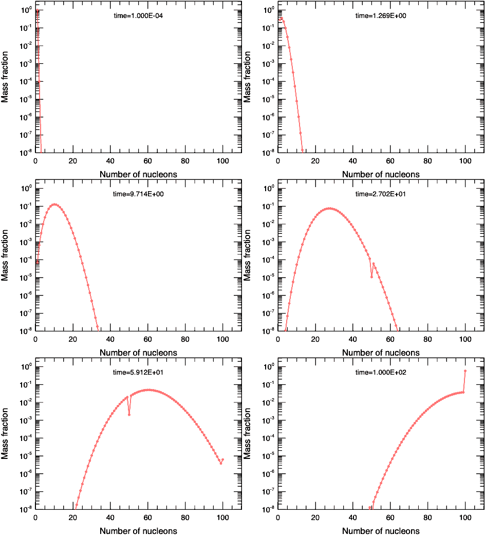The tool minis.tbz evolves an educational version of an s-process reaction network. One hundred isotopes are evolved until a chosen ending time. The initial abundance of the first isotope, notionally 56Fe, is taken equal to one. Guidance on what this tool does seems prudent. Let $R$ be the reaction rate for (n,g) reactions. In general $R$ is temperature, density, and composition dependent - but not here. The ordinary differential equations describing the change in the abundances $y$ of the $m$ isotopes are: \begin{equation} \frac{{\rm d}y_{1}}{{\rm d}t} = -y_{1} - R_{1} \hskip 0.5in \frac{{\rm d}y_{i}}{{\rm d}t} = y_{i-1} \ R_{i-1} - y_{i} \ R_{i} \ , \ i=1,2\ldots,m-1 \hskip 0.5in \frac{{\rm d}y_{m}}{{\rm d}t} = y_{m-1} \ R_{m-1} \label{eq1} \tag{1} \end{equation} For the implicit first-order accurate Euler method, each abundance is updated over a timestep h as $y_{i}^{{\rm new}} = y_{i} + \Delta y_{i}$. The change in the abundances over a time step $\Delta y_{i}$ is obtained from solving the system of linear equations $({\bf I}/h - \tilde{{\bf J}}) \cdot \Delta {\bf y} = \dot{\bf y}$, which is simply the familar $\tilde{{\bf A}} \cdot {\bf x} = {\bf b}$. With only (n,g) reactions, Jacobian matrix $\tilde{{\bf J}}$ has the simple form \begin{equation} \left[\begin{array}{rrrrrr} -R_{1} & & & & & \\ R_{1} & -R_{2} & & & & \\ & R_{2} & -R_{3} & & & \\ & & & \ldots & & \\ & & & & R_{m-1} & 0 \\ \end{array}\right] \label{eq2} \tag{2} \end{equation} This system of linear equations can be easily solved by hand: \begin{equation} \Delta y_1 = \frac{-y_1 R_1}{1/h + R_1} \hskip 0.5in \Delta y_i = \frac { y_{i-1} R_{i-1} - y_i R_i } {1/h + R_i} \ , \ i=1,2\ldots,m-1 \hskip 0.5in \Delta y_m = \frac{-y_{m-1} R_{m-1}}{1/h} \label{eq3} \tag{3} \end{equation} Thus the succint evolution loop implemented in minis.tbz. Here are some results: All exposures equal to one A middle exposure at 0.1 A middle exposure at 10.0
	Please cite the relevant references if you publish a piece of work that use these codes, pieces of these codes, or modified versions of them. Offer co-authorship of the publication if appropriate. At best, you'll love these programs so much that you'll send great wads of cash to me.